Samuel

0. Introduction

This blog post explains the main principles behind my recently released Scaffolding Generator. You can find a showcase video of it here on my Peertube channel. Due to the sheer number of nodes involved, I won't be able to explain everything to the finest detail. However, I still want to give you a broad overview of my thought process and how things work.

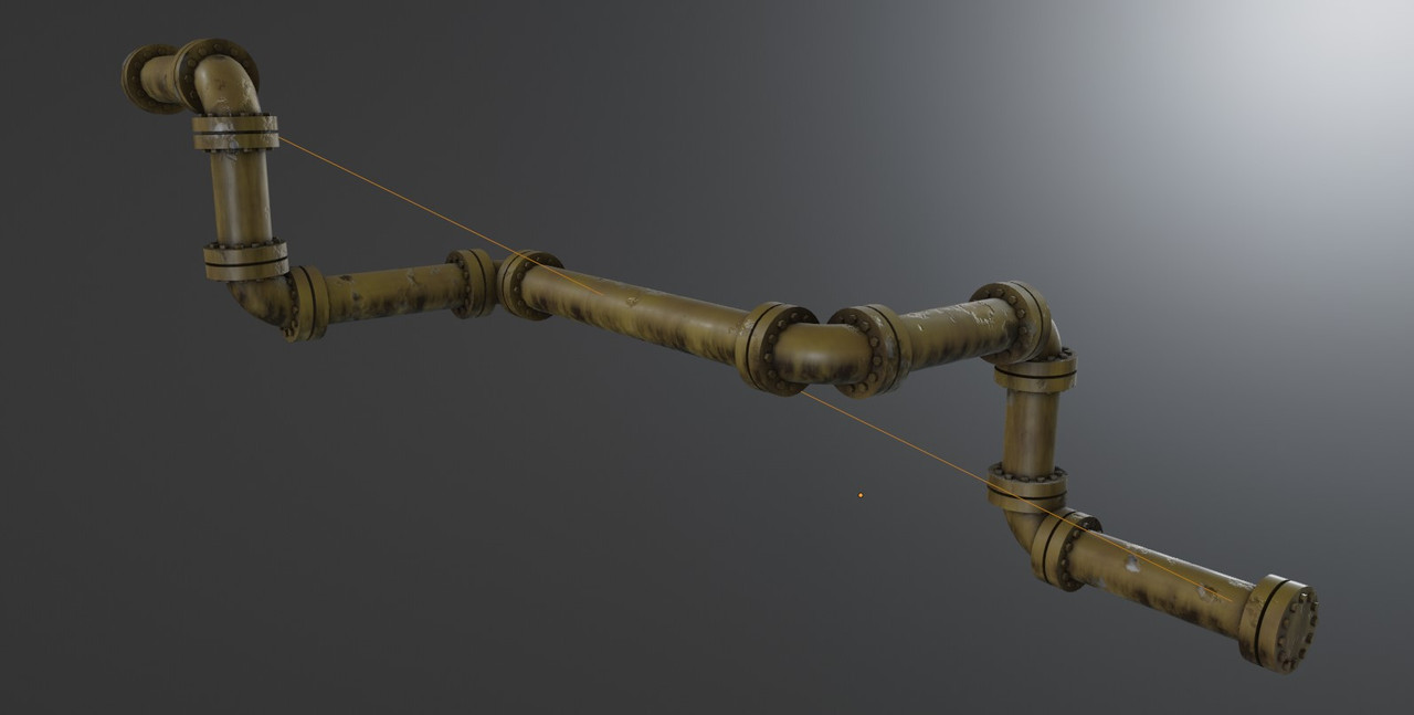
The base idea of the generator is simple. We feed it mesh edges, which are easy to move around and extrude, and out comes a scaffold. We want it to be able to adapt to corners. There should also be input parameters for the amount of floors, for their height and for the depth of the scaffold. With these inputs, we can control the generator from the modifiers tab without having to poke around in the geometry nodes graph. The scaffold should consist of floors (obviously) and of poles that connect everything in all three dimensions. Once that is figured out, we can move on to ladders and barriers and any other unnecessary detail that comes to mind.

When solving out complex problems like these, it is important to break them down into smaller and smaller problems until you can solve them bit by bit, but still keep the big picture in mind. So let's start building from the bottom up.

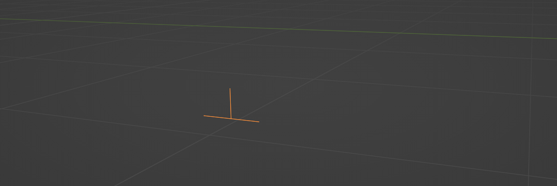
1. Creating a base floor

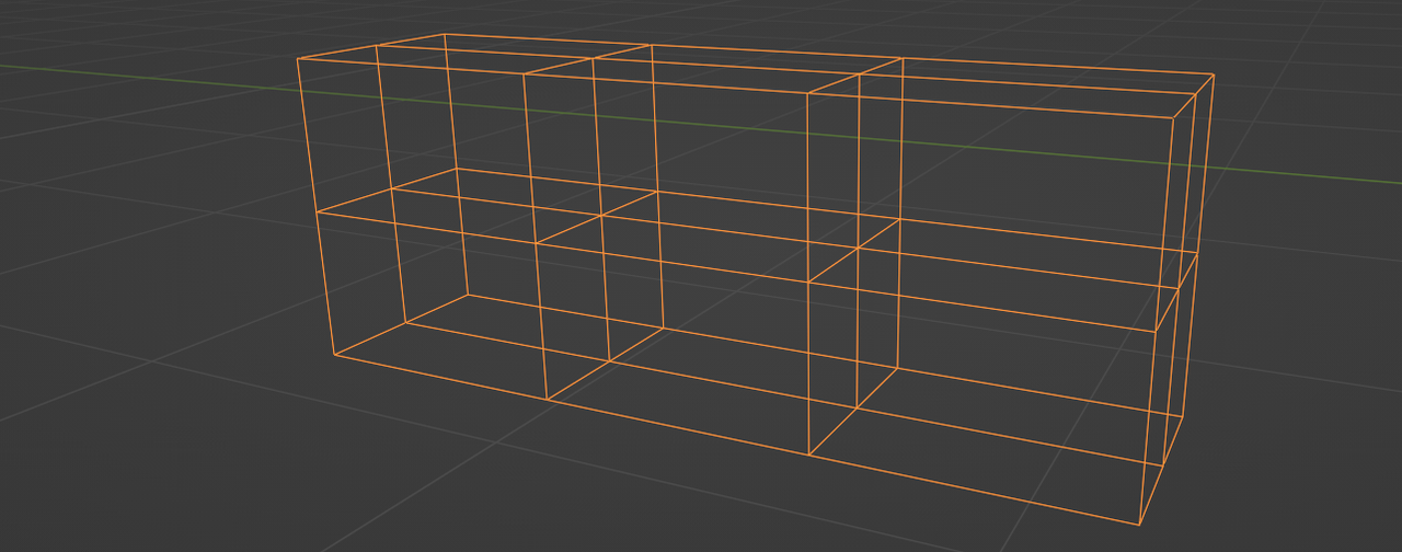
Scaffoldings are repetitive, so it makes sense to start with the most basic structure: a single floor. Our goal is to turn turn the input edges into a plane with parallel sides that resemble a floor.

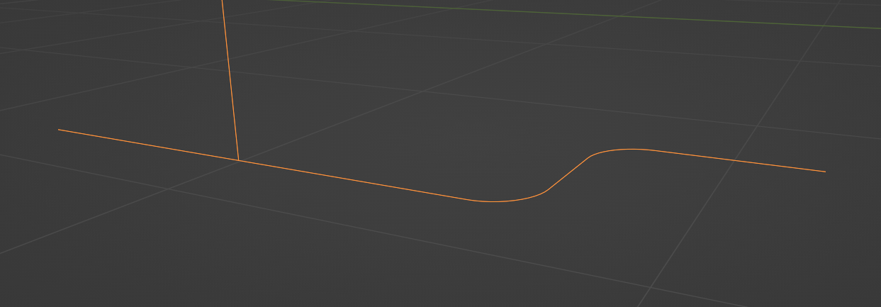
There's an easy way to extrude curves, and it's called “curve to mesh”. That means we first need to convert the input edges by using the “Mesh to Curves” modifier. Then all we have to use as the extrusion profile is a curve line that is rotated orthogonally to the direction of the input curve. The length of the profile curve corresponds to the width of our scaffold.

The result looks promising already. However, we can see that it messed up the corners; this is because the profile curve has been rotated by 45° at that point and not scaled accordingly. Thus, the extrusion ends up being too thin. Luckily for us there is a relatively easy fix for this, at least for angles between 90-180° (which is what we are interested in; most scaffoldings have >90° angles). You are free to dive down the rabbit hole by following this great tutorial by Blender Bash, but I will show an easier way here.

Since we're dealing with a curve as input, we can take advantage of the “set curve radius” node to scale every point of the curve according to the angle of its adjacent edges. Make sure to set the curve radius prior to doing the extrusion operation or this will not work. To access the angle between two curve segments, all we need to do is to calculate the dot product of its vectors like so:

Now let's use this dot product to adjust the curve radius. Remember, the absolute value of the dot product equals 0 for 90° angles and 1 for 180° angles. The base radius at every point along the curve is 1, and the adjusted radius at a 90° angle should equal 1.414. The keen reader will recognize this number, its the square root of 2. Assume a right triangle where the two adjacent sides are of length 1. Using good ol' Pythagoras, the length of the hypothenuse then equals the square root of 2 (or the sum of both sides squared). We could also go the accurate route and implement the following formula:

angle = acos(dot_product)
radius_adjustment = 1 / cos(angle / 2)

The easier but slightly inaccurate route, which I took, because I am lazy, is to use a Map Range node that turns the range 0 to 1 into a range of 1.414 to 1. Its a linear interpolation, but its close enough (and nobody will notice anyway).

To prevent the endpoints of the curve from being affected by this operation, simply run the radius adjustment through a Switch node with an Endpoint Selection as toggle. If a point either belongs to start or end, set the radius to 1. And that is how to adjust the radius at each point to create a (somewhat) even extrusion of our base floor.

2. Up we go

The base floor we just created will help us in two ways: 1) we can use it as actual floors if we manage to duplicate it upwards along the Z axis, and 2) we can extrude it to create the geometry that will later be turned into poles. Using our “Floor height” input parameter as the offset scale of the “Extrude Mesh” node, we can achieve something like this:

An easy way of creating arrays in geometry nodes is the Duplicate Elements node. We pass our number of floors into its Amount socket, und use the provided Duplicate Index to drive the offset. The Duplicate Elements node can work on any domain (points, edges, faces, etc), but here I chose the Instance domain. That means we first have to convert the incoming geometry into an instance. Because of this, we are then able to use “Translate Instances” with the Duplicate Index being responsible for the upwards translation. Multiply this with the Floor Height and we got ourselves a group that creates arrays along the Z axis:

Make sure to package these nodes into a group so we can then later repeat the process with other geometry (like the ladders).

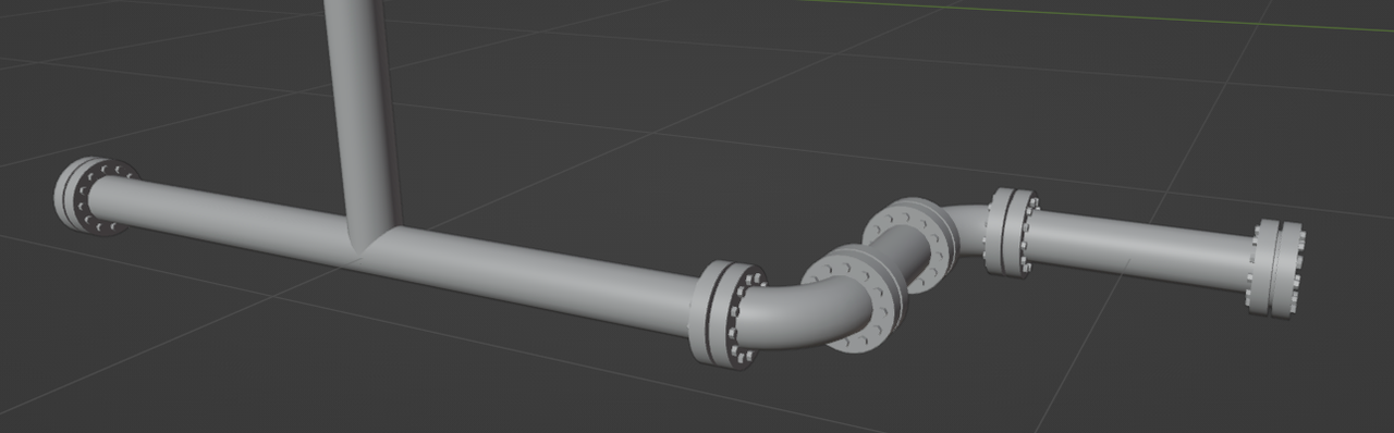
Time to turn our first prototype into poles. Same as with the ground floor, we use the “Curve to Mesh” modifier, but this time with a small curve circle as the profile. It's a good idea to wrap these nodes into their own group to re-use them for the ladders (I will call it the solidify group). Don't forget to turn your mesh into curves before the extrusion. The result should look like this:

3. Adding cuts

We can see that we need to add sections to our scaffold. Right now there are no subdivisions: the poles become as long as the base curve, and that's not really how scaffolds work. Time to move back to the early stages of our generator where we only have to deal with a few simple base curves. There is a “Subdivide Curve” modifier that allows us to set the amount of cuts we want to place inside a single curve. Right now, all the base curve segments are connected as a single curve, which means any cuts that we perform will be applied to the base curve as a whole. To treat every segment separately, we have to use “Split Edges” first, before our input edges are turned into the base curve. After splitting the edges, we capture an integer attribute that will control the amount of cuts. This attribute is calculated as follows:

• We first calculate the total length of each segment using the “Edge Vertices” positions, subtracting them from each other and calculating their length with a vector math node
• This length is then divided by a “Section length” input parameter that controls how long each section should be
• We floor the resulting value so that new cuts only spawn once a full section length is reached

If we now subdivide the curves according to our captured attribute, we will notice that they are not connected anymore; the extrusion operation will create two separate floor parts. That means we have to reconnect all individual curve segments that we split earlier. To do that, we turn our curve into a mesh again so that we can use the “Merge by Distance” modifier. As final step, we convert the merged mesh back into a curve. To summarize, the nodes will look like this:

4. Ladders

Okay, this part is going to be node so easy (I am not sorry). Let's first think about where we want to place ladders. We don't want to have ladders in every segment of our scaffold, but they should be placed in a regular distance along the base curve. That means we have to tell every segment of our base curve (after we subdivided it in section 3) whether or not a ladder should be placed on that position or not.

We can use the base curve to spawn ladders because of the “Mesh to Points” modifier, set to Edges. This modifier replaces all incoming edges with a point, on which we can then instance our ladders. And because “Instance on Points” allows us to pass it a selection as a Boolean value, we can store a Boolean attribute for each of the base edge to tell it whether a ladder should be spawned there or not. We do that after we subdivided our base curves and turned them into a mesh (aka edges) again. I call this attribute is_ladder. To get a repeating selection, we pass the Index of our edges into a modulo operation (for example with a modulo of 3), and compare the result with an integer (like 0). The result is a Boolean selection that is true for every third segment of our base curve.

Next comes the actual ladder. It should consist of two vertical poles, connected by a number of rungs. The height of the ladder should adapt to the floor height, and the amount of rungs should also adapt accordingly. The ladder should be tilted in an alternating pattern and spawn on every floor except for the topmost one. For the ladders we can re-use our solidify group to turn the curves into geometry. I can't explain every little detail of the ladder nodes here or this tutorial would never end, so let me try to summarize the steps:

• Create a single vertical curve line and set the X values of its start and end positions so that it is slightly tilted and adapts to the section length (the smaller the section length, the less the ladder is tilted).
• Resample the curve line based on the floor height (using a couple of math nodes).
• The created points of the curve can then be used to instance rungs (again just curve lines).
• Using our initial vertical curve line, we move it left and right by half the rung width to create the side poles of the ladder (and we join it with our instanced rungs).
• The resulting ladder consists only of curves for now, so we can scale it along the Y axis to adapt it to the width of our scaffold.
• Solidify the ladder curves to actual poles, using the solidify group we created earlier
• Stack the ladders using our floor stacking group (with the count being one less than the total floor count). The result is a single vertical stack of ladders.
• Every second of the resulting ladder instances is then rotated by 180°, driven by a floor_indexattribute that needs to be captured for every instance of the stacked ladders (inside our stacking group).
• After realizing the ladder instances, we can then instance the whole ladder stack on every point of our base curve (with the is_ladder selection applied).
• To rotate the ladder stacks according to the base curve, we need to store a curve tangent value for every base curve segment and pass it through an “Align Euler to Vector” node.

The result of our effort will look something like this:

5. Drawing the rest of the owl

There is certainly a lot more that can be done to further improve our little generator. However, I won't go into too much detail here anymore because most of the basic principles have been covered extensively, and many of the remaining details simply repeat the processes I've described earlier.

One of the more important aspects yet to do is to add those small outer offsets of the poles. Remember when we turned the mesh into curves that later became our poles? We can offset the start- and endpoints of these curves (separately) with the “Set Position” node with the help of the curve tangent attribute. The tangent is the vector that aligns with the direction of the curve. All we have to do is to normalize this tangent, so we don't end up with differently sized offsets, and use it as the offset of our “Set Position” node. You can then change the amount of offset by multiplying it with a small value.

Some scaffolds have diagonal poles in addition to the normal poles. We can create these using the “Triangulate” modifier. This operation must be performed on faces, i. e. right after we have extruded and stacked our floors.

To add barriers to the endpoints of our scaffold, we can again first create a single barrier object by manipulating curves (as we did with the ladders), solidify it with our solidify group, then stack it and instance these stacks on the endpoints of our base curve.

To add connector pieces where the poles intersect, we simple craft a little connector object with a small cylinder and a few extrusion and scaling operators, and then instance it on the vertices of the our stacked pole geometry. This should be done before we add the outer offsets of our poles, because we don't want to add the connectors at the very endpoints of our poles if they have offsets. We rotate the connectors according to the curve tangent.

And last but not least, we can offset each pole so that it won't intersect with its adjacent poles. It will look like the poles actually overlap each other instead of being directly connected. To offset each pole with a “Set Position” node, we first have to find a way to create a unique offset direction (or vector) for each pole curve. For this, I came up with a neat little idea: we create the cross product of two vectors, one being the face normal (the direction pointing away from the scaffold) and the other one being the curve tangent. The resulting vector points in a direction orthogonal to both of the other vectors. We capture the face normal and the curve tangent attributes with a “Capture Attribute” node set to the face and the point domains respectively. Bear in mind that the face normal needs to be captured before our extruded pole geometry is being turned into curves, i. e. while it still has face data. The captured vectors then need to be run through a Normalize and an Absolute step before being turned into the cross product.

I added a few more details like feet (simply instanced on the vertices of our base floor) and side panels (extrusions of the base floor with deleted upper and lower faces). The result looks like this:

And here is my abomination of a node graph:

6. Wrapping up

Well that was quite the ride, wasn't it? We started out with a single curve. We extruded it to form a base floor and fixed the corner width with completely inaccurate math tweaks. We extruded the base floor to generator pole geometry, which we then stacked to get a basic scaffold shape. We added diagonals and ladders and solidified everything to turn it into poles. At the end we merged our different branches of geometry together.

Thank you for taking the time to read my blog post to the end and I hope you learned a few things here and there. I am sure there exist smarter ways to do many of these operations, so hit me up on Mastodon with your thoughts and ideas. Critique and feedback is always welcome.

And now I wish you happy blendering!

Introduction

Pipes add detail and realism to 3D scenes, yet they are tedious to model manually and adapting them to scene changes is difficult. But thanks to the power of Blenders geometry nodes system, tasks like these can be automated with ease. In this blog post I will explain the concepts behind my pipe generator in detail. Bear in mind that I can't explain every step down to the individual node or this post would turn into a novel, and I'd rather use that time to work on other Blender projects. The post covers how to turn basic edges into pipes, how the automatic path finding works, what to consider when adding random offsets and finally I'll explain the hacky way I used to add junctions.

Water to wine, edges to pipes

Lets start with the basics: we need a node group that can turn any input edge into a pipe. Once we have this set up, we can later build upon it by adding the fancy stuff like path finding and special treatments for junctions.

The first thing to consider is the rounded curves. No pipe has straight corners, so we need to find a way to fillet them. Luckily there is a curve node that does just what we need: “Fillet Curve”. But we only want to fillet the corners, so we have to check whether the two edges are parallel to each other or not. This is where your vector math knowledge from school will come in handy: we're using the dot product of both edge directions. If the dot product is 1, the vectors are in a 90° angle to each other, if its 0, they're parallel. Use the “Field at index” position of the current index, the index -1 and the index +1 to find the edge directions.

Once this is done, there's two steps left for a basic pipe: turning it into a 3D mesh and adding the flanges. The first step is easy: simply use “Curve to Mesh” with a curve circle as profile. Adding the flanges is a bit harder. How do we determine on which points of the curve to instance the flanges? There might be better ways, but I did it with the “Attribute Statistics” node, using the edge length as input. We can assume that the tiny edges added by the filleting step are the shortest edges of the pipe, as well as the most common length statistically. We don't want to instance on those filleted corner vertices, just on the rest. So we create a selection where every edge larger than the median length is considered for flange instancing (for which we can use the “Instance on Points” node). On top of that we then add every vertex to the selection that has only 1 adjacent vertex. Why? Because we want the start and end points of our pipe to get flanges too.

How do we find the right direction in which to rotate the flanges? Easy, by capturing the curve tangent of the input edges and passing them to the “Rotate Instances” node via an “Align to Euler” node.

From 3D lettuce lattice to path

Now that we have a node group that turns every edge we throw at it into a pipe, it's time to start with the cool stuff: letting the math do the work for us.

If we want to create orthogonal paths that follow our input edges, we could use the “Shortest Edge Path” node. In conjunction with the “Edge Paths to Curves” node, we can pass selections for the end vertex and the start vertices to the path finding algorithm, which then tries to find a path through a mesh to connect these vertices, taking into account arbitrary edge cost values. That leaves us with two questions: how do we create a 3D lattice mesh around our input edges which the Shortest Edge Paths node can work in, and what do we use as edge cost?

To create a 3D edge lattice (there's plenty tutorials about that on YouTube) we simply create a 2D grid with the given X and Y dimensions and duplicate it upwards along the Z axis. The amount of subdivisions and duplications along the Z axis depend on the lattice resolution we need; I created a parameter that controls this resolution. As a last step for a basic 3D lattice we need the vertical edges: we instance upward-pointing curve lines on every vertex of the bottom-most grid, and divide the curve lines by the amount of grid rows on the Z axis. This subdivision step is required so we can use the “Merge by Distance” afterwards, which merges all vertices together.

Now that we have a generic 3D lattice, lets make it adapt to our input geometry. To do that, we use the “Convex Hull” node on our input geometry; it creates an enclosing mesh around all our input edges. We can then use the statistics of the positions of the convex hull vertices to change the scale of our 3D lattice and its offset in 3D space (otherwise we'd end up with a lattice that stays the same whatever we use as input geometry). For that we use the Range and Minimum values of the Attribute Statistic node.

To break the repetitive pattern of the lattice, we should offset the edges in random directions. But what happens if you offset a single edge of the lattice in a random direction? The adjacent edges won't be orthogonal anymore. To fix this, we have to move every row of each dimension as a whole. That means every edge in the X-Y plane would have to move in a random Z direction. To get a random value per row, we can use a noise texture with a one-dimensional vector as its input vector. Lets take the X dimension as an example. Our noise texture will only change in [1, 0, 0] space. We do the same for the other dimensions and combine them to a unified vector value (because its easier to pass on). We then capture this vector for every point on the lattice and let it drive the offset of the “Set Position” node. And et voilà, our lattice is no longer repetitive.

Time to move on to the Shortest Edge Path. How do we tell the path finding algorithm where to start and to end and where to draw the paths? To do that, we transfer the positions of our input edge start- and endpoints with the position of the “Sample Index” node to the “Sample Nearest” node that takes these positions and transfer them to the 3D lattice as its input geometry. The resulting selection contains the nearest vertices in the 3D lattice corresponding to our input edge start- and endpoints. And the edge cost? We simply use the distance value of the “Geometry Proximity” node to drive the edge cost. The farther a lattice edge is from the input edge, the less likely it is to be used by the path finding algorithm.

Junctions

What's left? I'm not a plumber, but I think whenever a pipe splits up into two sections, there needs to be a junction piece. How could we add this to our existing node graph? We already have a group that adds flanges at the end vertices of edges, so why not use that to our advantage?

First we have to select all junction vertices. Those can be found by checking how many vertex neighbours each vertex has. The most elegant way would then be to spawn N lines on each junction vertex, where N is the number of adjacent junction edges, and then capture the directions of said junction edges and rotate the instanced lines accordingly. I tried that ... and it didn't work, because I couldn't find a way to tell the node gods which rotation belongs to which instanced line; their indices are completely different from the indices of the junction edges.

So back to the scratch pad we go. What if we simply create a 6-way hedgehog of lines (one in each orthogonal direction; +/-X, +/-Y, +/-Z) on every junction vertex and then delete those of the lines that don't overlap with the pipe? Using the distance of the Geometry Proximity node, we can drive a Compare node and create a selection. Each of the hedgehog lines (what a silly name) whose distance is bigger than close to zero gets deleted. What remains are lines that align with our existing pipe paths and have a defined distance to our junction vertices. Of course this only works as long as the paths are orthogonal to each other, but its better than no junctions at all, I guess.

Conclusion

So there you have it, this is how I created my pipe generator. I had to cut a lot of corners in my explanation (or should I say, filleted?) but I hope you get the general idea of what's going on and could learn a thing or two about working with Geometry Nodes. If you want to try out the generator yourself or dissect my node graph, you can grab it here on Blendermarket for a few bucks. Happy blendering!